本文介绍单分子荧光漂白实验注意事项和台阶曲线提取以及自动化台阶计数方法。
单个荧光分子的光漂白过程可以通过单分子成像的方式记录下来,其荧光强度随时间变化具有一种阶梯状下降的特征。通过对曲线中包含的台阶进行计数,我们就能够知道在这个光斑的区域具体有几个荧光分子,因此这是一种先进且常见的分子计量方式。
单分子荧光漂白实验注意事项
采集到合格的单分子荧光漂白信号是大前提,由于是单分子成像实验,所以需要注意的地方还不少:
-
洁净的界面,例如0.17mm的硼硅酸盖玻片经过食人鱼溶液清洗后。
-
分子样品以合适的密度固定在界面上,一般来说 是比较合适的。
-
以较低的激光功率拍摄,基本能区分点状光斑和背景即可,不然有些荧光分子很快淬灭,导致台阶的长度过短而算法无法准确分析。
-
以较快的速度进行拍摄,最好是能在几分钟时间里结束战斗(以视野中所有荧光点消失为参考),不然界面的漂移会变得明显。
-
预览找焦面的视野不能采集数据,因为这个视野里的分子已经被「消耗」了一部分。找到焦面后要移动一些距离再采集数据。
-
由于照明不均,所以尽可能仅采集视野中央较小的区域,比如128x128像素范围内。
-
由于每个荧光分子实际能够发出的光子各不相同,所以同一个光斑位置存在多个荧光分子时,台阶曲线会逐渐变成指数衰减的曲线而变得难以分析,这也是这个分析方法的局限性。
单分子定位与台阶曲线批量提取
单分子成像拿到的原始数据,一般是 xyt 的视频形式。要分析台阶,首先就要提取某个光斑所在位置的荧光信号随时间变化曲线。这里可以使用 maxima 的方法找到这些 spot 的位置。
import osfrom glob import globimport numpy as npimport matplotlib.pyplot as pltfrom aicsimageio import AICSImage# pip install AICSImage[nd2]from skimage.morphology import h_maxima
# 读取目录下所有Nikon显微镜采集的原始数据fps = glob("*.nd2")
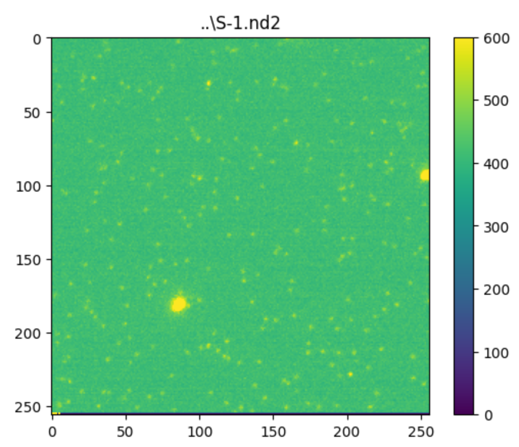
# 查看其中某一个数据def preview(fp): img = AICSImage(fp) frame = img.get_image_data("YX", T=0) plt.imshow(frame, vmin=0, vmax=600) plt.colorbar() plt.title(fp) plt.show()
fp = fps[0]fname = os.path.split(fp)[-1].split(".")[0]output_dir = fname+"_output"if not os.path.exists(fname+"_output"): os.mkdir(output_dir)preview(fp)上述代码我们写了一个简单的函数,来实现对数据的预览,看的就是第一帧的情况。并且根据这个数据创建好 output 存放目录,方便后面保存台阶曲线。
预览之后,接下来是要对这些 spot 进行定位。这里我采取的方式是对数据的前面若干帧进行平均强度投影,这样能够获得较好的信噪比,从而提高定位的准确性。
img = AICSImage(fp)mov = img.get_image_data('TYX')mip = mov[:100].mean(axis=0)plt.imshow(mip, vmax=600)plt.colorbar()plt.show()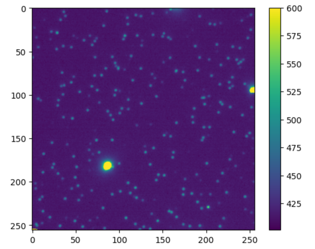
得到这个平均投影图像后,我们可以很容易地判断是否存在严重漂移的情况。如果漂移严重,这里点状光斑可能会变成其它的形状。既然数据质量OK,接下来可以使用 skimage.morphology.h_maxima 方法来进行单分子光斑的简单的像素定位(注意做超分辨的时候一般是用高斯拟合进行亚像素定位)。
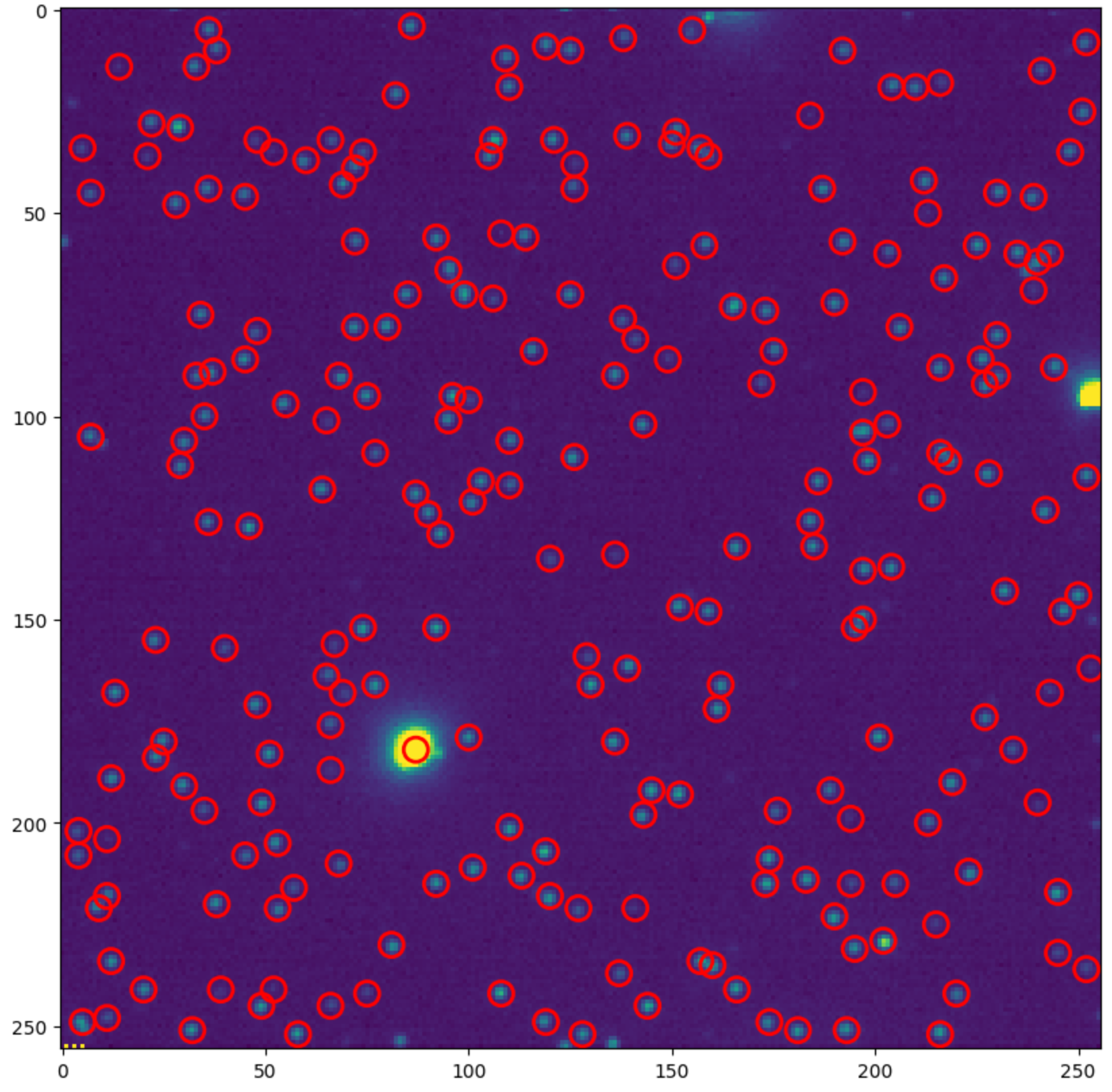
h_mask = h_maxima(mip, h=10)# h的数值可以从上班的colorbar的情况来进行调整# h_mask是一个二值化图像,有maxima的位置为1,其余为0rows, cols = np.where(h_mask==1)r = 3# 设定spot的像素半径,方便后面作图检查定位效果rmax, cmax = h_mask.shape
locs = []fig, ax = plt.subplots(figsize=(10,10))ax.imshow(mip, vmax=600)for y, x in zip(rows, cols): if x>=r and y>=r and x<=cmax-r and y<=rmax-r: # 去除边缘的spot c = plt.Circle((x, y), r, color='red', linewidth=2, fill=False) ax.add_patch(c) locs.append([x, y])plt.show()通过上述代码,可以实现基于 h_maxima 方法的单分子光斑像素位置的定位,这个位置信息收集到 locs 列表中。可以看到,定位的效果还是可以的(还可以根据spot的亮度进行简单的过滤):
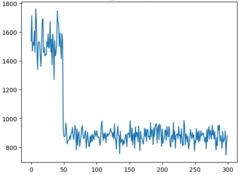
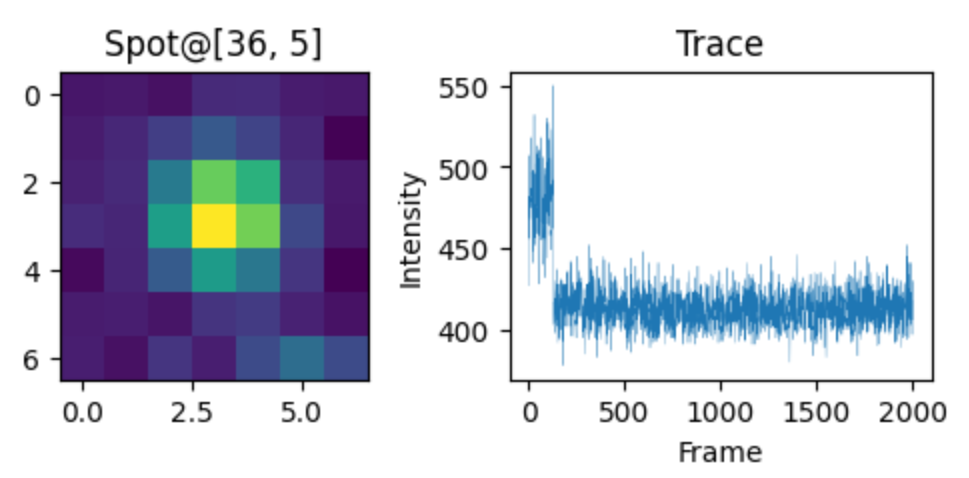
def showTrace(loc): zone = mip[loc[1]-3:loc[1]+4, loc[0]-3:loc[0]+4] trace = mov[:, loc[1], loc[0]] fig, axes = plt.subplots(figsize=(6,2), ncols=2) ax = axes.ravel() ax[0].imshow(zone) ax[0].set_title(f"Spot@{loc}") ax[1].plot(trace, linewidth=0.2) ax[1].set_title("Trace") ax[1].set_ylabel("Intensity") ax[1].set_xlabel("Frame") # plt.tight_layout() plt.show() return trace
# 查看光斑,trace并保存for idx, loc in enumerate(locs): trace = showTrace(loc) np.savetxt(os.path.join(output_dir, f"p_{idx}.txt"), trace)接下来,我们可以通过上边的自定义函数,在查看所有spot位置的 trace 的同时还把强度数据收集起来,直接保存到之前已经定义好的output目录下。
使用AutoStepfinder进行台阶分析
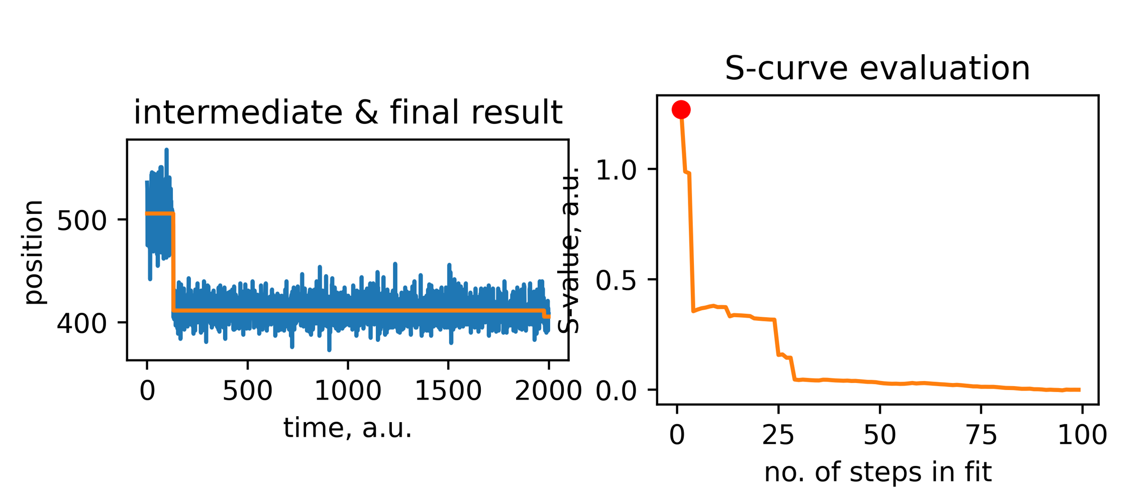
能够进行自动台阶分析的工具有一些,这里先介绍比较新,且不需要用户调整太多参数的 AutoStepfinder1。这个工具是2021年发表在Cell子刊 Patterns 上的,秉承着软件更新迭代会更优秀的经验,大部分情况下如果您的数据质量OK,使用这个会更加方便。这个工具以代码形式发布到了 github,并提供了 julia, matlib,python三种版本。此处我尝试了 python 版本,效果还可以。
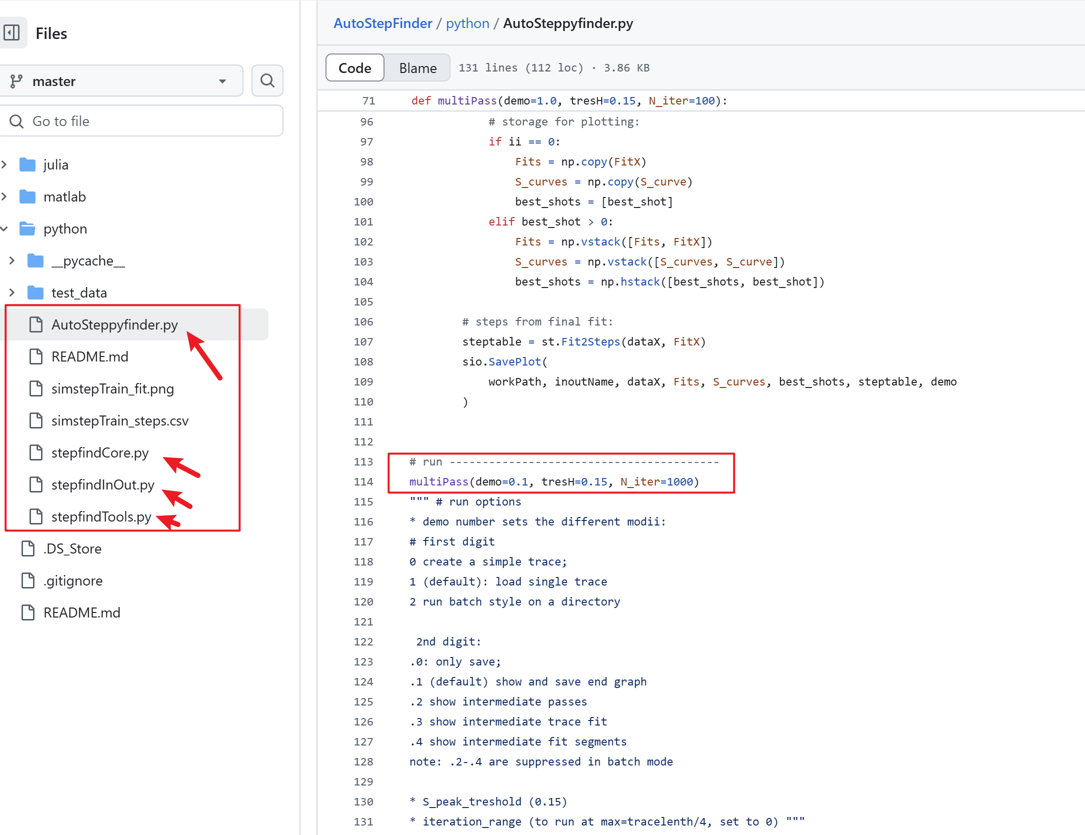
如上图所示,AutoStepfinder的核心代码就四个文件。实际使用时,值需要修改 multiPass函数中的三个参数(demo,tresH 和 N_iter)。
在实际进行批量分析的时候,demo=2.1,意味着对某个目录下所有trace数据进行分析,而且会同时保存台阶拟合的图以及台阶统计分析表格。然后 N_iter 最大就是trace长度的1/4 ,对于荧光漂白的数据,假如我采集了2000帧,绝大部分的荧光信号在200帧就已经漂白了,这里可以设置为 200。最后一个也是最重要 tresH,它是 S-Curve 的阈值设置,你可以简单地将它等价为数据的质量,数据质量越好,这个值可以设定得高一点。
结果表格如下:
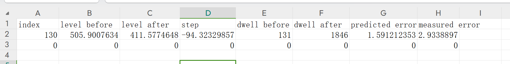
其中 index 就是这个台阶的索引位置,step就是台阶的高度,这里是负号说明是一个向下的台阶。level这是这个台阶前后的信号强度的值,dwell 就是台阶前后的长度。
使用Stepfinder进行台阶分析
在github上还能搜索到另外一个工具Stepfinder,这个是2019年发布的,相对来说需要调整的参数比较多,不过结果也更加准确。
代码下载下来后,注意因为年代比较久远了,所以最好使用 conda 新建一个 python 3.7或者3.8 的环境,然后安装相应比较低版本的 matplotlib,numpy 等模块,不然容易报错跑不起来。
我近期尝试的具体代码如下:
%matplotlib inline%config InlineBackend.figure_format='svg'import matplotlib.pyplot as pltimport numpy as npimport osfrom glob import globimport pandas as pdimport seaborn as snsimport syssys.path.append('..')import stepfinder as sf# https://github.com/tobiasjj/stepfinder/import warningswarnings.filterwarnings("ignore")
# 以下全是需要设定和调整的参数resolution = 20 # Hz, or fps
# Set parameters for filtering the data and finding stepsfilter_min_t = 0.1 # None or sfilter_max_t = 25 # None or sexpected_min_step_size = 25 # in values of data# expected_min_step_size = 50
# Set additional parameters for filtering the datafilter_time = 0.3 # None or sfilter_number = 5 # None or numberedginess = 1 # float
# Set additional parameters for finding the stepsexpected_min_dwell_t = 0.15 # None or sstep_size_threshold = 30 # None (equal to 'adapt'), 'constant', or in values of data为了方便查看参数调整后的影响,这是一段查看台阶拟合的效果的代码:
fp = glob('S-1_*\\p_26*.txt')[0]data = np.loadtxt(fp)
step_finder_result\ = sf.filter_find_analyse_steps(data, resolution, filter_time, filter_min_t, filter_max_t, filter_number, edginess, expected_min_step_size, expected_min_dwell_t, step_size_threshold, pad_data=True, verbose=False, plot=False)# Plot the data and step finder resultfig2, fig3 = sf.plot_result(step_finder_result)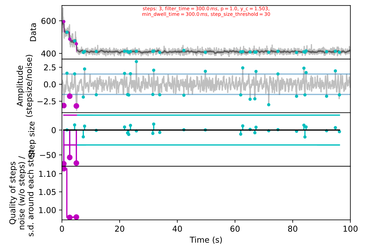
如果觉得参数调整好了,接下来可以批量处理:
def getBleachStepNumber(labels): # 光漂白时,应该是连续向下的台阶 # 初始化计数器 if len(labels)>0: count = 0 # 遍历列表,直到遇到第一个 True for item in labels: if item == False: count += 1 else: break return count else: return 0
def stepCounter(fp): data = np.loadtxt(fp) # 上方调好参数后整体复制到这里封装为函数,方便后面调用批量处理 resolution = 20 # Set parameters for filtering the data and finding steps filter_min_t = 0.1 # None or s filter_max_t = 25 # None or s expected_min_step_size = 25 # in values of data # expected_min_step_size = 50 # Set additional parameters for filtering the data filter_time = 0.3 # None or s filter_number = 5 # None or number edginess = 1 # float
# Set additional parameters for finding the steps expected_min_dwell_t = 0.15 # None or s step_size_threshold = 30 # None (equal to 'adapt'), 'constant', or in values of data step_finder_result\ = sf.filter_find_analyse_steps(data, resolution, filter_time, filter_min_t, filter_max_t, filter_number, edginess, expected_min_step_size, expected_min_dwell_t, step_size_threshold, pad_data=True, verbose=False, plot=False) n = getBleachStepNumber(step_finder_result.steps.direction) return n
box = {'type':[], 'sample':[], 'pid': [], 'x':[], 'y':[], 'n_step':[]}
for fp in fps: parts = os.path.split(fp) sample = parts[0] text = parts[-1] ps = text.split(".")[0].split("-") box['type'].append(stype) box['sample'].append(sample) box['pid'].append(int(ps[0].split("_")[-1])) box['x'].append(int(ps[1].split("_")[-1])) box['y'].append(int(ps[2].split("_")[-1])) box['n_step'].append(stepCounter(fp))
data = pd.DataFrame(box)# 完整的统计数据表,可以保存到表格文件,方便后续统计分析gp = data.groupby(by=['sample', 'n_step'])最后还可以作图检查台阶计数是否准确:
def checkProfile(idx): sample = data['sample'][idx] pid = data['pid'][idx] n_step = data['n_step'][idx] fp = fps[idx] curve = np.loadtxt(fp) plt.figure(figsize=(3,2)) plt.title(f'{sample}_{pid}: step={n_step}') plt.plot(curve) plt.show()
dat = gp.get_group(('S-1_output', 2))print(len(dat))for idx in dat.index: checkProfile(idx)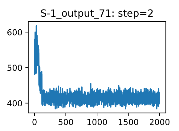
Footnotes
-
AutoStepfinder: A fast and automated step detection method for single-molecule analysis, Patterns, 2021. https://doi.org/10.1016/j.patter.2021.100256 ↩