使用编程的方式能够高度自定义地对大量数据进行分析,但为保证分析的准确性,需要对中间步骤进行充分的可视化检查。
由于实际采集的数据通常比较“脏”(即存在你没有考虑到的情况),所以如果基于少数抽样样本来设计算法并执行分析程序,大概率会得到错误的结果。如果分析结果奇怪还好,这会倒逼你回过头去逐步检查。最怕的是直接得出一个符合预期的结果。这里记录一个分析信噪比数据的案例。
from roifile import roireadfrom aicsimageio import AICSImagefrom skimage.draw import polygonimport os
import matplotlib.pyplot as pltimport pandas as pdimport numpy as np
def getFileList(wks, ext): '''ext 为文件后缀名''' flist = [] for root, ds, fs in os.walk(wks): for fname in fs: if fname.endswith(ext): fpath = os.path.join(root, fname) flist.append(fpath) return flist
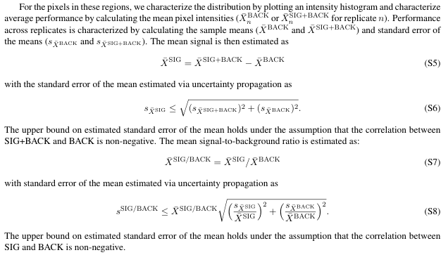
def get_values(img, roi): '''根据roi从图像中截取矩形范围''' coords = roi.coordinates() c = coords[:, 0] r = coords[:, 1] rows, cols = polygon(r, c) values = img[rows, cols].flatten() return values
def calculateSNR(a:list, b:list)->dict: ''' a: signal+background intensity b: background intensity ''' sig_bk = np.mean(a) bk = np.mean(b) sig = sig_bk - bk sig_bk_std = np.std(a) bk_std = np.std(b) sig_std = np.sqrt(pow(sig_bk_std, 2)+pow(bk_std, 2)) SNR = sig/bk SNR_std = SNR * np.sqrt(pow(sig_std/sig, 2) + pow(bk_std/bk, 2))
res = { "MEAN_SIG+BACK": sig_bk, "SD_SIG+BACK": sig_bk_std, "MEAN_BACK": bk, "SD_BACK": bk_std, "MEAN_SIG": sig, "SD_SIG": sig_std, "SNR": SNR, "SD_SNR": SNR_std, }
return res上述代码就包含了计算了信噪比的关键函数 calculateSNR,该方法来源于文献,需要同时输入信号的像素值(相机采集的信号区域,通常包含了背景),以及纯背景区域的像素值。然后采取均值相减的方式(sig_bk - bk = sig)获得实际的信号强度 sig,然后除以噪声均值 bk 得到信噪比 SNR。需要注意的是该方法默认噪声和信号的像素值都服从正态分布,所以选取ROI对信号和噪声的像素值进行采样时,注意避免人为偏误。
理论上上述代码能够完成SNR分析,但用户希望利用这个方法来实现细胞膜区域的一种特殊SNR分析,信号是他的方法增强的,而背景则是未使用该方法的对照组细胞膜区域的背景信号强度(存在细胞自发荧光的考虑)。这种基于指定object region从不同图像中采集sig和bk 的SNR分析也是可行的,出于描述简便,这种SNR分析本文简称为 cross-image SNR,然而因为数据量比较大,数据一致性就难以保证,所以就不得不进行必要的可视化。
[scode type=“yellow”]cross-image SNR分析的前提是成像参数都能保持一致,甚至要求拍摄时间都尽可能靠近,避免仪器状态的变化造成的影响[/scode]
fps = getFileList(wks='./', ext='czi')
df = {}
for idx, fp in enumerate(fps): n_channel = fp[2] # 多少色 pp = fp.split("\\") cell = pp[1] # 细胞类型 etype = pp[2] # 对照或实验组 rid = idx%2 + 1 # replicate次数 fp2 = fp.replace(".czi", ".rois.zip") rois = roiread(fp2) img = AICSImage(fp) pixelsize = img.physical_pixel_sizes.X channels = img.channel_names for idy, ch in enumerate(channels): ch_ = channel_alt[ch] if n_channel not in df: df[n_channel] = {} if cell not in df[n_channel]: df[n_channel][cell] = {} if etype not in df[n_channel][cell]: df[n_channel][cell][etype] = {} if rid not in df[n_channel][cell][etype]: df[n_channel][cell][etype][rid] = {} if ch_ not in df[n_channel][cell][etype][rid]: df[n_channel][cell][etype][rid][ch_] = {}
frame = img.get_image_data("YX", C=idy) bag = [] bbag = [] for idm, roi in enumerate(rois): values = get_values(frame, roi) if roi.roitype==1: bag.extend(values) elif roi.roitype==2: bbag.extend(values) df[n_channel][cell][etype][rid][ch_]['intensity'] = bag df[n_channel][cell][etype][rid][ch_]['background'] = bbag df[n_channel][cell][etype][rid][ch_]['rois'] = rois df[n_channel][cell][etype][rid][ch_]['img'] = frame df[n_channel][cell][etype][rid][ch_]['fp'] = fp df[n_channel][cell][etype][rid][ch_]['pixelsize'] = pixelsize为了便于可视化检查,那么从原始数据开始收集和提取的信息就要尽可能保持完整,而且要遵循一定的逻辑,如上述代码所示,我主要使用字典的方式来装载包含了不同颜色数量,不同细胞,不同实验组,重复组次数,以及成像通道的数据。然后每个数据是xy的frame,并且提取指定ROI(细胞膜区域)的像素,还保留了相关的各种信息,例如文件路径,像素尺寸,roi记录等等,都是为了方便可视化检查。
import matplotlib as mplimport matplotlib.colors as mcolorsmpl.rcParams['font.family'] = 'DengXian'plt.rcParams['axes.unicode_minus'] = False
def create_basic_colormap(color_name, num_colors=256): # 定义黄色范围的RGB值 bcmap = { 'red': (1, 0, 0), 'green': (0, 1, 0), 'blue': (0, 0, 1), 'yellow': (1, 1, 0), 'cyan': (0, 1, 1), 'purple': (1, 0, 1), 'gray': (1, 1, 1) } assert color_name in bcmap colors = [] color = bcmap[color_name] for i in range(num_colors): # 计算亮度值 (从0到1) brightness = i / (num_colors - 1) # 计算RGB值,注意保持色调,改变亮度 r = color[0] * brightness g = color[1] * brightness b = color[2] * brightness colors.append((r, g, b)) # 创建一个线性分段colormap cmap = mcolors.LinearSegmentedColormap.from_list(f"{color_name}_gradient", colors) return cmap
channel_alt = { 'ESID-T1': "BF", 'ESID-T2': "BF", 'AF488-T1': "488", "AF488-T2": "488", "AF594-T2": "568", "AF568-T1": "568", "AF610-T3": "647", "AF647-T3": "647",}
luts = { 'BF': create_basic_colormap('gray'), '488': create_basic_colormap('green'), '568': create_basic_colormap('yellow'), '647': create_basic_colormap('red'),}
def analyzeSNR(df, n_plex, cell_type, channel, replicate, vmin=0, vmax=2000): '''计算SNR的同时,显示图像和ROI n_plex = '2' cell_type = '97h' channel = '488' replicate = 2 vmin = 0 vmax = 2000 ''' cmap = luts[channel] a = df[n_plex][cell_type]['实验组'][replicate] b = df[n_plex][cell_type]['mock'][replicate] res_a = calculateSNR(a[channel]['intensity'], a[channel]['background']) res_b = calculateSNR(b[channel]['intensity'], b[channel]['background']) print(f"实验组 SNR: {res_a['SNR']:.2f}, Mock组 SNR: {res_b['SNR']:.2f}")
fig, ax = plt.subplots(ncols=2, nrows=2, figsize=(12,12))
ax[0,0].imshow(a[channel]['img'], cmap=luts[channel], vmin=vmin, vmax=vmax) ax[0,0].set_title("Exp"+f"\npixelsize: {a[channel]['pixelsize']:.3f} μm\n"+a[channel]['fp']) ax[1,0].imshow(a['BF']['img'], cmap=luts['BF']) rois = a[channel]['rois'] for roi in rois: if roi.roitype==1: cc = 'red' elif roi.roitype==2: cc = 'blue' pts = roi.coordinates() ax[0,0].fill(pts[:,0], pts[:,1], facecolor='none', edgecolor=cc, linewidth=1) ax[1,0].fill(pts[:,0], pts[:,1], facecolor='none', edgecolor=cc, linewidth=1)
ax[0,1].imshow(b[channel]['img'], cmap=cmap, vmin=vmin, vmax=vmax) ax[0,1].set_title("Mock"+f"\npixelsize: {b[channel]['pixelsize']:.3f} μm\n"+b[channel]['fp']) ax[1,1].imshow(b['BF']['img'], cmap=luts['BF']) rois = b[channel]['rois'] for roi in rois: if roi.roitype==1: cc = 'red' elif roi.roitype==2: cc = 'blue' pts = roi.coordinates() ax[0,1].fill(pts[:,0], pts[:,1], facecolor='none', edgecolor=cc, linewidth=1) ax[1,1].fill(pts[:,0], pts[:,1], facecolor='none', edgecolor=cc, linewidth=1)
plt.tight_layout() plt.show()
fig, ax = plt.subplots(ncols=2, nrows=1, figsize=(12,3)) ax = ax.ravel() ax[0].hist(a[channel]["intensity"], alpha=0.5, fc='red', ec='white', label='intensity', bins=30) ax[0].hist(a[channel]["background"], alpha=0.5, fc='blue', ec='white', label='background', bins=30) ax[0].set_xlabel("Pixel Value") ax[0].set_ylabel("Pixel Count") ax[0].legend() ax[1].hist(b[channel]["intensity"], alpha=0.5, fc='red', ec='white', label='intensity', bins=30) ax[1].hist(b[channel]["background"], alpha=0.5, fc='blue', ec='white', label='background', bins=30) ax[1].set_xlabel("Pixel Value") ax[1].set_ylabel("Pixel Count") ax[1].legend() plt.tight_layout() plt.show() res = { '实验组': res_a['SNR'], 'mock': res_b['SNR'] } return res可视化检查分析的代码就会变得非常复杂。如上述代码所示,为了使用合适伪彩显示细胞图像,还得先自定义一段代码(后面可以封装起来,作为自己常用的代码模块进行 import);然后用户原始数据中channel name 比较乱,经确认是同一个channel,所以还写了一个 channel_alt 的字典方便做规范化,以便后面批量处理。同时再通过一个 luts 的字典,方便自动给不同的 channel 上合适的伪彩。
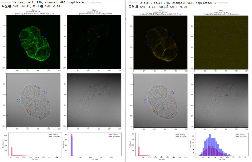
由于数据一致性无法保证,所以在 analyzeSNR 函数中,我只能是对每张图自身的信噪比进行分析,这种可以称之为 local SNR。然后每次 analyzeSNR,则会对指定条件和细胞的实验组和对照组数据分别计算 local SNR,然后显示细胞指定通道荧光图像和明场图像,sig 和 bk的ROI区域,原始文件路径,pixelsize等等信息,方便检查。
n_plex = '2'cell = '97h'channel = '488'replicate = 1print(f"====== {n_plex}-plex, cell: {cell}, channel: {channel}, replicate: {replicate} ======")res = analyzeSNR(df, n_plex, cell, channel, replicate, vmin=0, vmax=5000)封装好函数之后,具体的调用如上述代码所示,结果如下图:
总之,数据可视化是保证数据分析结果准确性的必要检查手段。