要判断一个东西是否在一个三维区域的内部还是外部是很简单的,但是要直观地展示出来这种三维空间的内外关系,需要一些技巧。这里举个例子。
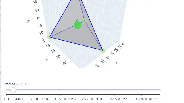
先看结果:
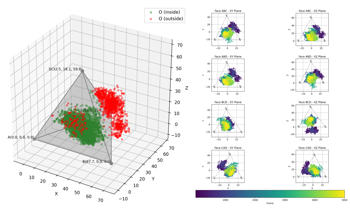
如上图所示,目标分子使用散点表示,如果在四面体内部则标记为绿色,如果在外部则标记为红色。这样能够已经能够比较好地表示内外的情况了。但是pdf不像html支持三维查看,所以三维只能看到某一个视角,就容易产生视觉上的误差。
因此更准确详细的做法,可以是计算这些点在四面体上各个面上的投影情况。即以四面体每个面作为新的局部坐标系的xy平面,然后坐标系z轴正放下给指向四面体内部,x轴方向和指定棱保持一直,局部坐标系的原点为这个面三角形的几何中心。然后完成点坐标在不同局部坐标系的映射即可。此外二维作图的时候,还可以使用折线表示点的轨迹,折线的颜色表示点的时间。
然后三维和二维的作图相结合,就可以把时空关系充分地直观地展示出来。
把上述需求稍微整理细化,丢给grok:
写一个python函数:函数输入是一个pd.DataFrame,包含这些列:Frame,O_x,O_y,O_z,A_x,A_y,A_z,B_x,B_y,B_z,C_x,C_y,C_z,D_x,D_y,D_z。每一行代表O、A、B、C、D五个点在特定时间帧的空间坐标。ABCD四个点组成了一个四面体。以下是函数内部要做的事情:1. 对所有时间点的A,B,C,D四个点的坐标求平均,从而得到平均四面体ABCD,这个平均四面体的坐标可使用字典存储其四个点坐标,是返回值之一。2. 以平均四面体ABCD上的面ABC创建一个局部直角坐标系,这个局部直角坐标系的原点是面的几何中心,局部直角坐标系的z轴方向就是这个面的朝向四面体内部的方向,局部直角坐标系的x轴与AB平行且方向相同,局部直角坐标系的y轴的方向则朝向C点一侧。3. 建立好这样一个局部直角坐标系后,计算五个点在所有时间点上的坐标在这个新的局部直角坐标系的投影坐标,请注意规范命名变量以存储新的坐标,以O点为例,新的坐标为 O_x_ABC, 后缀ABC表示局部直角坐标系的xy平面。4. 以平均四面体ABCD上的面ABD创建一个局部直角坐标系,这个局部直角坐标系的原点是面的几何中心,局部直角坐标系的z轴方向就是这个面的朝向四面体内部的方向,局部直角坐标系的x轴与AB平行且方向相同,局部直角坐标系的y轴的方向则朝向D点一侧。5. 建立好这样一个局部直角坐标系后,计算五个点在所有时间点上的坐标在这个新的局部直角坐标系的投影坐标,请注意规范命名变量以存储新的坐标,以O点为例,新的坐标为 O_x_ABD, 后缀ABD表示局部直角坐标系的xy平面。6. 以平均四面体ABCD上的面BCD创建一个局部直角坐标系,这个局部直角坐标系的原点是面的几何中心,局部直角坐标系的z轴方向就是这个面的朝向四面体内部的方向,局部直角坐标系的x轴与BC平行且方向相同,局部直角坐标系的y轴的方向则朝向D点一侧。7. 建立好这样一个局部直角坐标系后,计算五个点在所有时间点上的坐标在这个新的局部直角坐标系的投影坐标,请注意规范命名变量以存储新的坐标,以O点为例,新的坐标为 O_x_BCD, 后缀BCD表示局部直角坐标系的xy平面。8. 以平均四面体ABCD上的面CAD创建一个局部直角坐标系,这个局部直角坐标系的原点是面的几何中心,局部直角坐标系的z轴方向就是这个面的朝向四面体内部的方向,局部直角坐标系的x轴与CA平行且方向相同,局部直角坐标系的y轴的方向则朝向D点一侧。9. 建立好这样一个局部直角坐标系后,计算五个点在所有时间点上的坐标在这个新的局部直角坐标系的投影坐标,请注意规范命名变量以存储新的坐标,以O点为例,新的坐标为 O_x_CAD, 后缀CAD表示局部直角坐标系的xy平面。10. 将上述计算得到的所有坐标作为新增列添加到输入的 pd.DataFrame,作为函数的返回值之一。通过少量测试和修改,就实现了这样的坐标系变化。接下来就是对结果进行可视化。这个迭代修改的次数比较多,所以就不放记录了,感兴趣的大家自己看我分享的grok聊天记录吧。
该功能的输入(数据表)是之前一篇文章的输出。
代码如下:
import pandas as pdimport numpy as npfrom glob import globimport matplotlib.pyplot as pltfrom matplotlib.collections import LineCollectionfrom mpl_toolkits.mplot3d import Axes3Dfrom matplotlib import cmfrom mpl_toolkits.mplot3d.art3d import Poly3DCollection
def process_tetrahedron_coordinates(df): """ Process tetrahedron coordinates and compute projections in local coordinate systems.
Parameters: df (pd.DataFrame): Input DataFrame with columns Frame, O_x, O_y, O_z, A_x, A_y, A_z, B_x, B_y, B_z, C_x, C_y, C_z, D_x, D_y, D_z
Returns: tuple: (mean_tetrahedron, result_df) - mean_tetrahedron: dict with mean coordinates of points A, B, C, D - result_df: DataFrame with original data and new projected coordinates """ # 1. Calculate mean coordinates for points A, B, C, D mean_tetrahedron = { 'A': np.array([df['A_x'].mean(), df['A_y'].mean(), df['A_z'].mean()]), 'B': np.array([df['B_x'].mean(), df['B_y'].mean(), df['B_z'].mean()]), 'C': np.array([df['C_x'].mean(), df['C_y'].mean(), df['C_z'].mean()]), 'D': np.array([df['D_x'].mean(), df['D_y'].mean(), df['D_z'].mean()]) }
# Initialize result DataFrame result_df = df.copy()
# Define faces and their corresponding configurations faces = [ ('ABC', ['A', 'B', 'C'], ['A', 'B'], 'C'), ('ABD', ['A', 'B', 'D'], ['A', 'B'], 'D'), ('BCD', ['B', 'C', 'D'], ['B', 'C'], 'D'), ('CAD', ['C', 'A', 'D'], ['C', 'A'], 'D') ]
def create_local_coordinate_system(face_points, x_axis_points, y_side_point, mean_tetrahedron): """Create local coordinate system for a face.""" # Get mean coordinates p1, p2, p3 = [mean_tetrahedron[p] for p in face_points]
# Calculate face center (origin) origin = (p1 + p2 + p3) / 3
# Calculate normal vector (z-axis) pointing inside tetrahedron v1 = p2 - p1 v2 = p3 - p1 normal = np.cross(v1, v2) # Ensure normal points inside tetrahedron to_center = mean_tetrahedron[list(set(['A', 'B', 'C', 'D']) - set(face_points))[0]] - origin if np.dot(normal, to_center) > 0: normal = -normal z_axis = normal / np.linalg.norm(normal)
# x-axis along first edge x_axis = mean_tetrahedron[x_axis_points[1]] - mean_tetrahedron[x_axis_points[0]] x_axis = x_axis / np.linalg.norm(x_axis)
# y-axis perpendicular to x and z, towards y_side_point y_axis = np.cross(z_axis, x_axis) to_y_point = mean_tetrahedron[y_side_point] - origin if np.dot(y_axis, to_y_point) < 0: y_axis = -y_axis y_axis = y_axis / np.linalg.norm(y_axis)
# Create transformation matrix transform_matrix = np.vstack([x_axis, y_axis, z_axis]).T
return origin, transform_matrix
def project_coordinates(coordinates, origin, transform_matrix): """Project coordinates to local coordinate system.""" # Translate to origin and project translated = coordinates - origin projected = np.dot(translated, transform_matrix) return projected[:, 0], projected[:, 1], projected[:, 2]
# Process each face for face_name, face_points, x_axis_points, y_side_point in faces: # Create local coordinate system origin, transform_matrix = create_local_coordinate_system( face_points, x_axis_points, y_side_point, mean_tetrahedron )
# Project coordinates for all points (O, A, B, C, D) for point in ['O', 'A', 'B', 'C', 'D']: coords = df[[f'{point}_x', f'{point}_y', f'{point}_z']].values x_new, y_new, z_new = project_coordinates(coords, origin, transform_matrix)
# Add new coordinates to result DataFrame result_df[f'{point}_x_{face_name}'] = x_new result_df[f'{point}_y_{face_name}'] = y_new result_df[f'{point}_z_{face_name}'] = z_new
return mean_tetrahedron, result_df
def visualize_tetrahedron_projections(results_df, sample): """ Create a 4x2 grid of plots for visualizing tetrahedron point projections. For each face, plot the mean coordinates of the three face points as a triangle with labeled vertices in xy-plane, and a different triangle in xz-plane. Point O is plotted as a colored line based on Frame order. All axes have equal scale. XZ-plane z-coordinates are transformed to positive. Each subplot's axis range is adjusted to center the triangle. No legend is shown. Colorbar is displayed at the bottom.
Parameters: results_df (pd.DataFrame): DataFrame containing projected coordinates with columns like O_x_ABC, O_y_ABC, O_z_ABC, etc.
Returns: None (saves figure as 'tetrahedron_projections.png') """ # Define face suffixes, titles, and points for each face (xy and xz planes) faces = [ ('ABC', 'Face ABC', ['A', 'B', 'C'], ['A', 'B', 'D']), ('ABD', 'Face ABD', ['A', 'B', 'D'], ['A', 'B', 'C']), ('BCD', 'Face BCD', ['B', 'C', 'D'], ['B', 'C', 'A']), ('CAD', 'Face CAD', ['C', 'A', 'D'], ['A', 'B', 'C']) ]
# Create 4x2 subplot grid fig, axes = plt.subplots(4, 2, figsize=(12, 16)) plt.subplots_adjust(hspace=0.4, wspace=0.3, bottom=0.15) # Adjust bottom for colorbar
# Get colormap for point O's line cmap = plt.get_cmap('viridis')
for row, (face_suffix, face_title, xy_points, xz_points) in enumerate(faces): # Get axes for this row ax_xy = axes[row, 0] ax_xz = axes[row, 1]
# Calculate mean coordinates for xy-plane points mean_coords_xy = { point: { 'x': results_df[f'{point}_x_{face_suffix}'].mean(), 'y': results_df[f'{point}_y_{face_suffix}'].mean() } for point in xy_points }
# Calculate mean coordinates for xz-plane points (z transformed to positive) mean_coords_xz = { point: { 'x': results_df[f'{point}_x_{face_suffix}'].mean(), 'z': -results_df[f'{point}_z_{face_suffix}'].mean() # Negate z } for point in xz_points }
# Calculate axis ranges for xy-plane to center the triangle xy_x_coords = [mean_coords_xy[p]['x'] for p in xy_points] + list(results_df[f'O_x_{face_suffix}']) xy_y_coords = [mean_coords_xy[p]['y'] for p in xy_points] + list(results_df[f'O_y_{face_suffix}']) xy_x_min, xy_x_max = np.min(xy_x_coords), np.max(xy_x_coords) xy_y_min, xy_y_max = np.min(xy_y_coords), np.max(xy_y_coords) xy_x_range = xy_x_max - xy_x_min xy_y_range = xy_y_max - xy_y_min xy_range = max(xy_x_range, xy_y_range) * 1.2 # Add 20% padding xy_x_center = (xy_x_max + xy_x_min) / 2 xy_y_center = (xy_y_max + xy_y_min) / 2
# Calculate axis ranges for xz-plane to center the triangle xz_x_coords = [mean_coords_xz[p]['x'] for p in xz_points] + list(results_df[f'O_x_{face_suffix}']) xz_z_coords = [mean_coords_xz[p]['z'] for p in xz_points] + list(-results_df[f'O_z_{face_suffix}']) xz_x_min, xz_x_max = np.min(xz_x_coords), np.max(xz_x_coords) xz_z_min, xz_z_max = np.min(xz_z_coords), np.max(xz_z_coords) xz_x_range = xz_x_max - xz_x_min xz_z_range = xz_z_max - xz_z_min xz_range = max(xz_x_range, xz_z_range) * 1.2 # Add 20% padding xz_x_center = (xz_x_max + xz_x_min) / 2 xz_z_center = (xz_z_max + xz_z_min) / 2
# Plot triangle for xy-plane triangle_xy = np.array([ [mean_coords_xy[p]['x'] for p in xy_points + [xy_points[0]]], [mean_coords_xy[p]['y'] for p in xy_points + [xy_points[0]]] ]).T ax_xy.plot(triangle_xy[:, 0], triangle_xy[:, 1], 'gray', alpha=0.5)
# Plot triangle for xz-plane (z transformed to positive) triangle_xz = np.array([ [mean_coords_xz[p]['x'] for p in xz_points + [xz_points[0]]], [mean_coords_xz[p]['z'] for p in xz_points + [xz_points[0]]] ]).T ax_xz.plot(triangle_xz[:, 0], triangle_xz[:, 1], 'gray', alpha=0.5)
# Plot and label mean points for xy-plane for point in xy_points: ax_xy.scatter( mean_coords_xy[point]['x'], mean_coords_xy[point]['y'], c='gray', alpha=0.7 ) ax_xy.text( mean_coords_xy[point]['x'], mean_coords_xy[point]['y'], point, fontsize=8, ha='right', va='bottom' )
# Plot and label mean points for xz-plane (z transformed) for point in xz_points: ax_xz.scatter( mean_coords_xz[point]['x'], mean_coords_xz[point]['z'], c='gray', alpha=0.7 ) ax_xz.text( mean_coords_xz[point]['x'], mean_coords_xz[point]['z'], point, fontsize=8, ha='right', va='bottom' )
# Plot point O as a colored line based on Frame order norm = plt.Normalize(results_df['Frame'].min(), results_df['Frame'].max()) points_xy = np.array([ results_df[f'O_x_{face_suffix}'], results_df[f'O_y_{face_suffix}'] ]).T points_xz = np.array([ results_df[f'O_x_{face_suffix}'], -results_df[f'O_z_{face_suffix}'] # Negate z for O ]).T segments_xy = np.array([points_xy[:-1], points_xy[1:]]).transpose(1, 0, 2) segments_xz = np.array([points_xz[:-1], points_xz[1:]]).transpose(1, 0, 2)
# Create line collections for colored lines lc_xy = LineCollection( segments_xy, cmap=cmap, norm=norm ) lc_xz = LineCollection( segments_xz, cmap=cmap, norm=norm )
# Set line colors based on Frame lc_xy.set_array(results_df['Frame'][:-1]) lc_xz.set_array(results_df['Frame'][:-1])
# Add line collections to plots ax_xy.add_collection(lc_xy) ax_xz.add_collection(lc_xz)
# Set titles and labels ax_xy.set_title(f'{face_title} - XY Plane') ax_xz.set_title(f'{face_title} - XZ Plane') ax_xy.set_xlabel('X' if row == 3 else '') ax_xz.set_xlabel('X' if row == 3 else '') ax_xy.set_ylabel('Y') ax_xz.set_ylabel('Z')
# Set equal aspect ratio and centered axis ranges ax_xy.set_aspect('equal') ax_xz.set_aspect('equal') ax_xy.set_xlim(xy_x_center - xy_range / 2, xy_x_center + xy_range / 2) ax_xy.set_ylim(xy_y_center - xy_range / 2, xy_y_center + xy_range / 2) ax_xz.set_xlim(xz_x_center - xz_range / 2, xz_x_center + xz_range / 2) ax_xz.set_ylim(xz_z_center - xz_range / 2, xz_z_center + xz_range / 2)
# Add grid ax_xy.grid(True) ax_xz.grid(True)
# Add colorbar at the bottom cbar = fig.colorbar( cm.ScalarMappable(norm=norm, cmap=cmap), ax=axes, location='bottom', fraction=0.05, pad=0.04, label='Frame' )
# Save the figure plt.savefig(f'{sample}_2d_projections.png', dpi=300, bbox_inches='tight') plt.close()
def visualize_mean_tetrahedron(mean_tetrahedron, results_df, sample): """ Create a 3D plot of the mean tetrahedron. Points A, B, C, D are plotted as gray scatter points with labels including coordinates. Tetrahedron surfaces are gray with transparency (alpha=0.7). Edges are solid gray lines. Point O is plotted as scatter points, green if inside the tetrahedron, red if outside.
Parameters: mean_tetrahedron (dict): Dictionary with mean coordinates for points A, B, C, D (e.g., {'A': [x, y, z], 'B': [x, y, z], ...}) results_df (pd.DataFrame): DataFrame containing O_x, O_y, O_z coordinates
Returns: None (saves figure as 'mean_tetrahedron_3d.png') """ # Create figure and 3D axes fig = plt.figure(figsize=(8, 8)) ax = fig.add_subplot(111, projection='3d')
# Extract coordinates for A, B, C, D points = np.array([mean_tetrahedron[p] for p in ['A', 'B', 'C', 'D']]) x, y, z = points[:, 0], points[:, 1], points[:, 2]
# Define tetrahedron faces (vertices for each face) faces = [ [points[0], points[1], points[2]], # ABC [points[0], points[1], points[3]], # ABD [points[1], points[2], points[3]], # BCD [points[2], points[0], points[3]] # CAD ]
# Define edges (all unique pairs of points) edges = [ (0, 1), # A-B (0, 2), # A-C (0, 3), # A-D (1, 2), # B-C (1, 3), # B-D (2, 3) # C-D ]
# Function to compute barycentric coordinates def barycentric_coordinates(p, tetra_points): a, b, c, d = tetra_points T = np.array([b - a, c - a, d - a]).T try: bary = np.linalg.solve(T, p - a) # Append the first coordinate (1 - sum of others) bary = np.append(bary, 1 - np.sum(bary)) return bary except np.linalg.LinAlgError: # If singular matrix, return invalid coordinates return np.array([-1, -1, -1, -1])
# Extract O coordinates o_points = np.array([results_df['O_x'], results_df['O_y'], results_df['O_z']]).T
# Determine if O points are inside or outside inside = [] for o in o_points: # Compute barycentric coordinates bary = barycentric_coordinates(o, points) # Point is inside if all barycentric coordinates are in [0, 1] and sum to ~1 is_inside = np.all(bary >= -1e-10) and np.all(bary <= 1 + 1e-10) and abs(np.sum(bary) - 1) < 1e-10 inside.append(is_inside)
inside = np.array(inside) results_df['inside'] = inside
# Plot scatter points for A, B, C, D ax.scatter(x, y, z, c='gray', s=50)
# Add labels for points with coordinates (rounded to 1 decimal place) for i, point in enumerate(['A', 'B', 'C', 'D']): coords = mean_tetrahedron[point] label = f"{point}({coords[0]:.1f}, {coords[1]:.1f}, {coords[2]:.1f})" ax.text(points[i][0], points[i][1], points[i][2], label, fontsize=8, ha='right', va='bottom')
# Plot scatter points for O (green for inside, red for outside) ax.scatter(o_points[inside][:, 0], o_points[inside][:, 1], o_points[inside][:, 2], c='green', s=15, label='O (inside)', alpha=0.1) ax.scatter(o_points[~inside][:, 0], o_points[~inside][:, 1], o_points[~inside][:, 2], c='red', s=15, label='O (outside)', alpha=0.1)
# Plot tetrahedron surfaces with transparency poly = Poly3DCollection(faces, facecolors='gray', alpha=0.2, edgecolors='none') ax.add_collection3d(poly)
# Plot edges for edge in edges: edge_points = points[list(edge)] ax.plot(edge_points[:, 0], edge_points[:, 1], edge_points[:, 2], 'gray', linewidth=1.5)
# Set labels ax.set_xlabel('X') ax.set_ylabel('Y') ax.set_zlabel('Z')
# Set equal aspect ratio ax.set_box_aspect([1, 1, 1])
# Calculate axis limits to center the tetrahedron and O points all_points = np.vstack([points, o_points]) all_coords = [all_points[:, i] for i in range(3)] min_vals = np.min(all_coords, axis=1) max_vals = np.max(all_coords, axis=1) ranges = max_vals - min_vals max_range = np.max(ranges) * 1.2 # Add 20% padding centers = (max_vals + min_vals) / 2 ax.set_xlim(centers[0] - max_range / 2, centers[0] + max_range / 2) ax.set_ylim(centers[1] - max_range / 2, centers[1] + max_range / 2) ax.set_zlim(centers[2] - max_range / 2, centers[2] + max_range / 2)
# Add grid ax.grid(True)
# Add legend for O points ax.legend(loc='upper right')
# Save the figure plt.savefig(f'{sample}_3d-view-in-out.png', dpi=300, bbox_inches='tight') plt.close() return results_df
def main(): fps = glob("out/*.csv") for fp in fps: df = pd.read_csv(fp) sample = fp.split(".")[0] tdn, df2 = process_tetrahedron_coordinates(df) df2 = visualize_mean_tetrahedron(tdn, df2, sample) visualize_tetrahedron_projections(df2, sample) df2.to_excel(f'{sample}_results.xlsx', index='Frame')
if __name__=='__main__': main()